BBN Generation

BBN generation is available in py-scm. We support singly- and multi-connected Gaussian BBNs.

Singly-connected BBN

Use generate_singly_gaussian_bbn() to generate a singly-connected Gaussian BBN and then use create_reasoning_model() to create a reasoning model.

This example uses max_iter=20 so the generated tree is more illustrative than the initial ordered chain.

from help.viz import get_graph_layout, to_networkx
import matplotlib.pyplot as plt
import networkx as nx
from pyscm.generator import generate_singly_gaussian_bbn
from pyscm.reasoning import create_reasoning_model

generated = generate_singly_gaussian_bbn(
    n=10,
    max_iter=20,
    seed=37,
    max_degree=3,
    max_condition_number=25.0,
)

g = generated.graph
p = generated.parameters

model = create_reasoning_model(g, p)

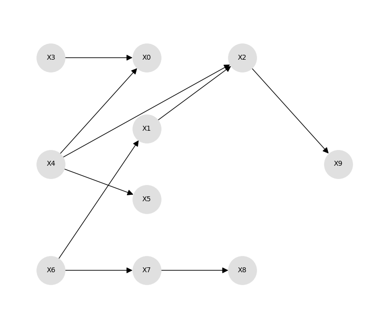
The singly-connected BBN graph looks like the following.

dag = to_networkx(g)

fig, ax = plt.subplots(figsize=(8.0, 6.75))

pos = get_graph_layout(dag, seed=37)
nx.draw(
    dag,
    pos=pos,
    with_labels=True,
    node_color="#e0e0e0",
    node_size=1700,
    font_size=10,
    arrows=True,
    arrowsize=18,
    ax=ax,
)

ax.margins(x=0.10, y=0.18)
fig.tight_layout()

Posterior queries proceed as usual.

means, covariance = model.pquery({"X1": 0.5}, pandas=True)
means.to_frame("mean")

	mean
X0	0.448743
X1	0.500000
X2	0.235416
X3	-0.670662
X4	-0.602994
X5	-0.064449
X6	0.261791
X7	0.194697
X8	-0.158753
X9	0.323203

model.iquery("X9", {"X1": 1.25}, pandas=True)

mean    0.346223
std     0.445736
dtype: float64

Multi-connected BBN

Use generate_multi_gaussian_bbn() to generate a multi-connected Gaussian BBN and then use create_reasoning_model() to create a reasoning model.

This example also uses max_iter=20, and the fixed seed below keeps the example reproducible while avoiding a near-chain structure.

from pyscm.generator import generate_multi_gaussian_bbn

generated = generate_multi_gaussian_bbn(
    n=10,
    max_iter=20,
    seed=3,
    max_degree=4,
    intercept_mean=0.25,
    intercept_sd=0.2,
    weight_mean=0.0,
    weight_sd=0.3,
    noise_sd_min=0.4,
    noise_sd_max=0.8,
    max_condition_number=25.0,
)

g = generated.graph
p = generated.parameters

model = create_reasoning_model(g, p)

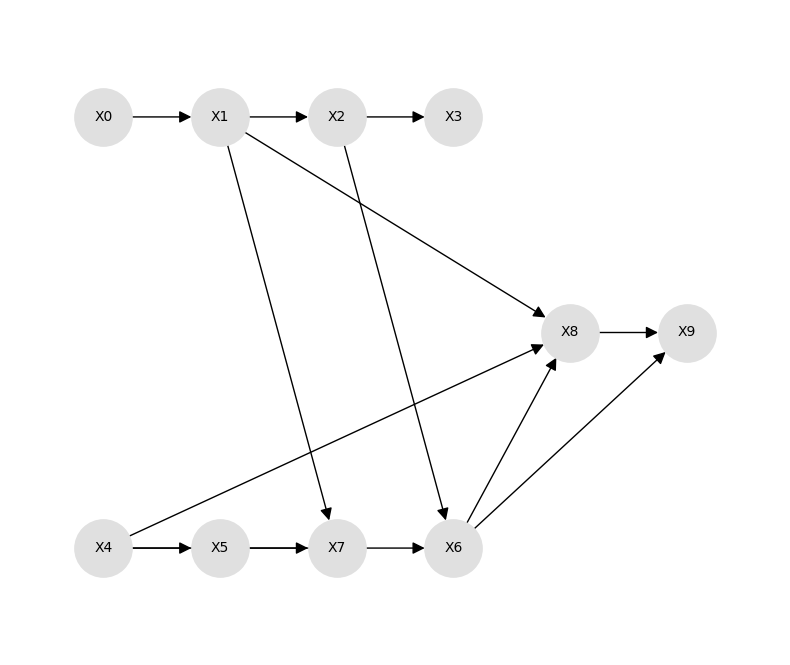
The multi-connected BBN graph looks like the following.

dag = to_networkx(g)

fig, ax = plt.subplots(figsize=(8.0, 6.75))

pos = get_graph_layout(dag, seed=37)
nx.draw(
    dag,
    pos=pos,
    with_labels=True,
    node_color="#e0e0e0",
    node_size=1700,
    font_size=10,
    arrows=True,
    arrowsize=18,
    ax=ax,
)

ax.margins(x=0.10, y=0.18)
fig.tight_layout()

model.equery("X9", {"X1": 1.0}, {"X1": -1.0}, pandas=True)

mean   -0.065951
std     0.000000
dtype: float64

model.samples(size=10).head()

	X0	X1	X2	X3	X4	X5	X6	X7	X8	X9
0	-0.556711	1.441756	1.197602	1.866988	1.280589	1.494780	0.098026	-1.253835	1.353719	-0.212623
1	-0.197582	0.442962	0.409467	0.598435	0.287417	-0.534240	-0.379872	-0.264745	-0.311271	-1.134408
2	0.932308	-0.675724	0.050717	-0.025196	1.192979	0.476395	0.155484	0.517682	0.180630	1.389682
3	0.999141	0.412904	0.997719	0.746910	1.027509	-0.066919	0.186078	-0.061389	-0.409386	0.091236
4	0.063324	0.269446	0.948745	0.565484	0.967308	-0.756124	-0.774144	-0.307976	-0.050875	1.624334