Learning Tree Structures
Causal tree structures are easier to understand than general structures since the graph is sparse. Let’s see how to learn a tree structure with py-scm.
Causal model
The true causal model is defined as follows.
\(X_1 \sim \mathcal{N}(1, 1)\)
\(X_2 \sim \mathcal{N}(2.3, 1)\)
\(X_3 \sim \mathcal{N}(1 + 2 X_1 - 4 X_2, 1)\)
\(X_4 \sim \mathcal{N}(5 - 8.5 X_3, 2)\)
\(X_5 \sim \mathcal{N}(8 + 2.5 X_3, 1)\)
We have already simulated data from this causal model, and so we will load it.
[1]:
import pandas as pd

X = pd.read_csv('./_data/tree.csv')
X.shape
[1]:
(10000, 5)
[2]:
X.head(10)
[2]:
| X1 | X2 | X3 | X4 | X5 | |
|---|---|---|---|---|---|
| 0 | 1.794997 | 2.317933 | -3.517468 | 30.910707 | 0.460451 |
| 1 | 0.998971 | 2.740944 | -9.924201 | 89.787225 | -17.754713 |
| 2 | 2.015391 | 2.734284 | -5.535403 | 48.127835 | -6.642635 |
| 3 | 2.529683 | 1.569960 | -1.218079 | 13.999461 | 5.018192 |
| 4 | 0.701551 | 1.803381 | -3.139628 | 30.856091 | 0.071788 |
| 5 | 0.137326 | 4.565585 | -17.735502 | 161.393584 | -35.437648 |
| 6 | 0.450718 | 1.270369 | -3.962104 | 40.005610 | -2.699435 |
| 7 | 0.667200 | 1.326497 | -2.935497 | 25.938894 | 0.777087 |
| 8 | 2.187346 | 3.126029 | -7.770064 | 69.013016 | -12.026722 |
| 9 | 0.558971 | 3.744352 | -13.587705 | 120.293070 | -27.265520 |
Tree algorithm
Let’s apply the tree structure learning algorithm to try and recover the causal model.
[3]:
from pyscm.learn import Tree

algorithm = Tree().fit(X)
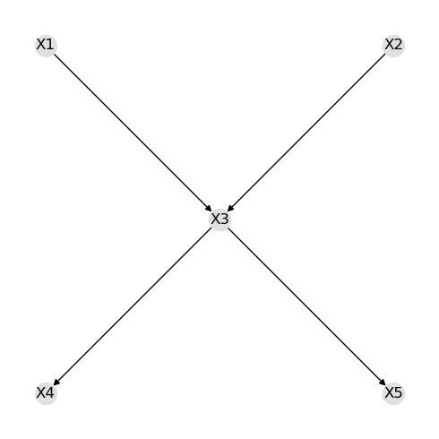
As you can see below, the true structure is recovered.
[4]:
import networkx as nx
import matplotlib.pyplot as plt

fig, ax = plt.subplots(figsize=(5, 5))

g = algorithm.g
pos = nx.nx_agraph.graphviz_layout(g, prog='dot')
nx.draw(g, pos=pos, with_labels=True, node_color='#e0e0e0')

fig.tight_layout()
The means and covariance matrix are available.
[5]:
algorithm.m
[5]:
X1     0.996357
X2     2.295660
X3    -6.173479
X4    57.460345
X5    -7.442364
dtype: float64
[6]:
algorithm.c
[6]:
| X1 | X2 | X3 | X4 | X5 | |
|---|---|---|---|---|---|
| X1 | 1.007207 | 0.019826 | 1.937162 | -16.488629 | 4.852801 |
| X2 | 0.019826 | 1.009765 | -3.996842 | 33.985064 | -9.988840 |
| X3 | 1.937162 | -3.996842 | 20.855450 | -177.370103 | 52.147059 |
| X4 | -16.488629 | 33.985064 | -177.370103 | 1512.468328 | -443.495280 |
| X5 | 4.852801 | -9.988840 | 52.147059 | -443.495280 | 131.370791 |
Reasoning model
A py-scm reasoning model may then be created as follows.
[7]:
from pyscm.reasoning import create_reasoning_model

model = create_reasoning_model(algorithm.d, algorithm.p)
model
[7]:
ReasoningModel[H=[X1,X2,X3,X4,X5], M=[0.996,2.296,-6.173,57.460,-7.442], C=[[1.007,0.020,1.937,-16.489,4.853]|[0.020,1.010,-3.997,33.985,-9.989]|[1.937,-3.997,20.855,-177.370,52.147]|[-16.489,33.985,-177.370,1512.468,-443.495]|[4.853,-9.989,52.147,-443.495,131.371]]]
We can then use the associational, interventional and counterfactual inference capabilities of the reasoning model.
Associational query
Here is an associational query without evidence.
[8]:
q = model.pquery()
[9]:
q[0]
[9]:
X1     0.996357
X2     2.295660
X3    -6.173479
X4    57.460345
X5    -7.442364
dtype: float64
[10]:
q[1]
[10]:
| X1 | X2 | X3 | X4 | X5 | |
|---|---|---|---|---|---|
| X1 | 1.007207 | 0.019826 | 1.937162 | -16.488629 | 4.852801 |
| X2 | 0.019826 | 1.009765 | -3.996842 | 33.985064 | -9.988840 |
| X3 | 1.937162 | -3.996842 | 20.855450 | -177.370103 | 52.147059 |
| X4 | -16.488629 | 33.985064 | -177.370103 | 1512.468328 | -443.495280 |
| X5 | 4.852801 | -9.988840 | 52.147059 | -443.495280 | 131.370791 |
Here’s another associational query with evidence.
[11]:
q = model.pquery({'X1': 5})
[12]:
q[0]
[12]:
X1     5.000000
X2     2.374468
X3     1.526735
X4    -8.081902
X5    11.847503
dtype: float64
[13]:
q[1]
[13]:
| X1 | X2 | X3 | X4 | X5 | |
|---|---|---|---|---|---|
| X1 | 1.007207 | 0.019826 | 1.937162 | -16.488629 | 4.852801 |
| X2 | 0.019826 | 1.009375 | -4.034973 | 34.309628 | -10.084363 |
| X3 | 1.937162 | -4.034973 | 17.129702 | -145.657488 | 42.813657 |
| X4 | -16.488629 | 34.309628 | -145.657488 | 1242.538686 | -364.051759 |
| X5 | 4.852801 | -10.084363 | 42.813657 | -364.051759 | 107.989613 |
Interventional query
What happens with the distribution when we do an interventional query?
[14]:
model.iquery('X4', {'X3': 5})
[14]:
mean   -37.640420
std      0.056625
dtype: float64
Counterfactual query
Lastly, here’s some counterfactual queries.
Given we observed the following,
\(X_1=1\),
\(X_2=2.3\),
\(X_3=-6.1\),
\(X_4=58\), and
\(X_5=-8\),
what would of happened to \(X_3\) had the following occured?
\(X_1=1\)
\(X_1=2\)
\(X_1=3\)
\(X_1=2, X_2=3\)
[15]:
f = {
    'X1': 1,
    'X2': 2.3,
    'X3': -6.1,
    'X4': 58,
    'X5': -8
}

cf = [
    {'X1': 1},
    {'X1': 2},
    {'X1': 3},
    {'X1': 2, 'X2': 3}
]

q = model.cquery('X3', f, cf)
[16]:
q
[16]:
| X1 | X2 | factual | counterfactual | |
|---|---|---|---|---|
| 0 | 1 | 2.3 | -6.1 | -6.100000 |
| 1 | 2 | 2.3 | -6.1 | -4.101476 |
| 2 | 3 | 2.3 | -6.1 | -2.102952 |
| 3 | 2 | 3.0 | -6.1 | -6.908138 |