Learning
Structure and parameter learning with py-scm is possible. Let’s show how to use py-scm to learn a causal model using the PC-algorithm.
Causal model
The true causal model is defined as follows.
\(C \sim \mathcal{N}(1, 1)\)
\(X \sim \mathcal{N}(1 + 2 C, 1)\)
\(M \sim \mathcal{N}(5 + 1.5 X, 1)\)
\(Y \sim \mathcal{N}(1 + 2 C + 1.5 X + 0.5 M, 1)\)
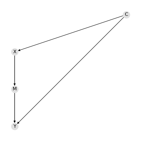
As you can see,
\(C\) is a confounder of \(X\) and \(Y\), and
\(M\) is a mediator between \(X\) and \(Y\).
We have already simulated data from this causal model, and so we will load it.
[1]:
import pandas as pd

X = pd.read_csv('./_data/model.csv')
X.shape
[1]:
(10000, 4)
[2]:
X.head(10)
[2]:
| C | X | M | Y | |
|---|---|---|---|---|
| 0 | 0.945536 | 3.024955 | 9.759877 | 10.532426 |
| 1 | 1.674308 | 3.387163 | 10.893335 | 15.800990 |
| 2 | 1.346647 | 3.589577 | 10.983322 | 13.636408 |
| 3 | -0.300346 | 0.253631 | 4.309610 | 2.124186 |
| 4 | 2.518512 | 4.986335 | 12.109710 | 18.424847 |
| 5 | 1.989824 | 6.312251 | 13.992190 | 23.169803 |
| 6 | 1.277681 | 1.963059 | 7.153576 | 9.272288 |
| 7 | 0.551411 | 1.834353 | 7.416663 | 9.534964 |
| 8 | 1.961966 | 2.707050 | 7.871503 | 13.247716 |
| 9 | 0.172421 | 1.636739 | 8.839026 | 8.404960 |
PC-algorithm
Let’s apply the PC-algorithm to try and recover the causal model.
[3]:
from pyscm.learn import Pc

algorithm = Pc().fit(X)
As you can see below, the true structure is recovered.
[4]:
import networkx as nx
import matplotlib.pyplot as plt

fig, ax = plt.subplots(figsize=(5, 5))

g = algorithm.g
pos = nx.nx_agraph.graphviz_layout(g, prog='dot')
nx.draw(g, pos=pos, with_labels=True, node_color='#e0e0e0')

fig.tight_layout()
The means and covariance matrix are available.
[5]:
algorithm.m
[5]:
C     1.001723
X     2.994276
M     9.496402
Y    12.231968
dtype: float64
[6]:
algorithm.c
[6]:
| C | X | M | Y | |
|---|---|---|---|---|
| C | 0.990700 | 1.989244 | 2.994101 | 6.461545 |
| X | 1.989244 | 5.004194 | 7.532975 | 15.238727 |
| M | 2.994101 | 7.532975 | 12.324022 | 23.445529 |
| Y | 6.461545 | 15.238727 | 23.445529 | 48.496009 |
Reasoning model
A py-scm reasoning model may then be created as follows.
[7]:
from pyscm.reasoning import create_reasoning_model

model = create_reasoning_model(algorithm.d, algorithm.p)
model
[7]:
ReasoningModel[H=[C,X,M,Y], M=[1.002,2.994,9.496,12.232], C=[[0.991,1.989,2.994,6.462]|[1.989,5.004,7.533,15.239]|[2.994,7.533,12.324,23.446]|[6.462,15.239,23.446,48.496]]]
We can then use the associational, interventional and counterfactual inference capabilities of the reasoning model.
[8]:
q = model.pquery()
[9]:
q[0]
[9]:
C     1.001723
X     2.994276
M     9.496402
Y    12.231968
dtype: float64
[10]:
q[1]
[10]:
| C | X | M | Y | |
|---|---|---|---|---|
| C | 0.990700 | 1.989244 | 2.994101 | 6.461545 |
| X | 1.989244 | 5.004194 | 7.532975 | 15.238727 |
| M | 2.994101 | 7.532975 | 12.324022 | 23.445529 |
| Y | 6.461545 | 15.238727 | 23.445529 | 48.496009 |